Link: Separating mixed signals with ICA
Implementation of Independent Components Analysis
Import packages
1
2
3
4
5
import numpy as npimport matplotlib.pyplot as plt%matplotlib inline from scipy import signalfrom tqdm.notebook import tqdm
Generate the source \(S\)
\(S\in R^d\)
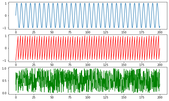
Here we choose 3 sources of signals: sine, sawtooth and noise.
1
2
3
4
5
6
7
8
9
10
11
12
13
f = plt.figure(figsize = (10 ,6 )) ax = f.add_subplot(311 ) ax2 = f.add_subplot(312 ) ax3 = f.add_subplot(313 ) t = np.linspace(0 , 200 , 1000 ) sine = np.sin(t) sawtooth = signal.sawtooth(t*1.9 ) noise = np.random.random(len(t)) ax.plot(t, sine) ax2.plot(t, sawtooth, 'r' ) ax3.plot(t, noise, 'g' ) plt.show()
1
2
S = np.vstack((sine, sawtooth, noise)) S.shape
(3, 1000)Mixture Matrix A, \(x = As\)
\(s_j^{(i)} = w_j^Tx^{(i)}\)
\(x^{(i)} = As^{(i)}\)
1
2
3
4
5
A = np.array([ [0.5 ,1 ,0.2 ], [1 ,0.5 ,0.4 ], [0.5 ,0.8 ,1 ] ])
array([[-0.3 , 1.4 , -0.5 ],
[ 1.33333333, -0.66666667, 0. ],
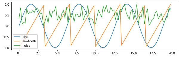
[-0.91666667, -0.16666667, 1.25 ]])1 2 3 4 5 6 7 plt.figure(figsize=(10 ,3 )) plt.plot(t[:100 ], sine[:100 ]) plt.plot(t[:100 ], sawtooth[:100 ]) plt.plot(t[:100 ], noise[:100 ]) plt.legend(labels = ["sine" , "sawtooth" , "noise" ]) plt.show()
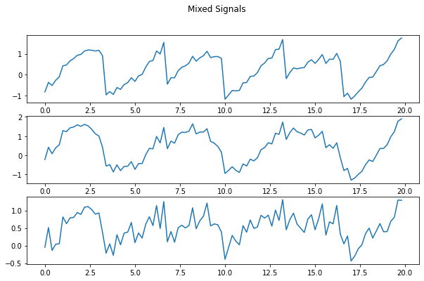
1 2 3 4 5 6 7 8 9 10 11 f = plt.figure(figsize=(10 ,6 )) f.suptitle("Mixed Signals" ) ax1 = f.add_subplot(311 ) ax2 = f.add_subplot(312 ) ax3 = f.add_subplot(313 ) ax1.plot(t[:100 ], X[0 ][:100 ]) ax2.plot(t[:100 ], X[1 ][:100 ]) ax3.plot(t[:100 ], X[2 ][:100 ]) plt.show()
ICA Algorithm
1 2 3 4 5 6 7 8 9 def center (x ): return x - np.mean(x, axis=1 , keepdims=True ), np.mean(x, axis=1 , keepdims=True ) def covariance (x ): mean = np.mean(x, axis=1 , keepdims=True ) n = np.shape(x)[1 ] - 1 m = x - mean return m.dot(m.T) / n
1 2 3 4 5 6 7 8 def whiten (x ): cov = covariance(x) U,S,V = np.linalg.svd(cov) d = np.diag(1 / np.sqrt(S)) whiteM = np.dot(U, np.dot(d, U.T)) Xw = np.dot(whiteM, X) return Xw, whiteM
1 2 def sigmoid (x ): return 1 / (1 + np.exp(-x))
1 2 3 4 5 6 7 8 def update (W, xi, lr ): """ Stochastic gradient ascent, one point xi """ gradient = np.dot((1 - 2 * sigmoid(np.dot(W.T, xi))), xi.T) + np.linalg.inv(W.T) diff = np.abs(gradient).sum() return W + lr*gradient, diff
1 2 3 4 5 6 7 8 9 10 def optimize (X, S, lr=0.1 , thresh=1e-2 , iterations=1000000 ): d, n = S.shape W = np.random.random(size=(d,d)) for c in tqdm(range(iterations)): xi = X[:,np.random.randint(0 ,n-1 )] W, diff = update(W, xi, lr) if (diff < thresh): break return W
1 2 3 4 5 6 Xc, meanX = center(X) Xw, whiteM = whiten(Xc) W_ = optimize(Xw,S) unMixed = Xw.T.dot(W_.T) unMixed = (unMixed.T - meanX)
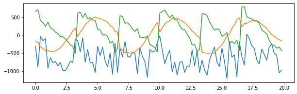
1 2 3 4 5 6 plt.figure(figsize=(10 ,3 )) plt.plot(t[:100 ], unMixed[0 ][:100 ]) plt.plot(t[:100 ], unMixed[1 ][:100 ]) plt.plot(t[:100 ], unMixed[2 ][:100 ]) plt.show()
The ICA ambiguities tells us that there is no way to recover the scaling of the wi's