(11/3) PCA中的centering的目的是?
- 注意到我们对于协方差矩阵的表达式 \(\Sigma = XX^T, X\in \mathbb{R}^{N\times d}\)
- 实际上的协方差表达式 \(Cov(X) = E[XX^T] - E[X] (E[X])^T\)
- 所以需要centering各分量
(11/3) PCA中特征值为什么对应方差贡献量?
- 对\(\Sigma\) 这个半正定对称矩阵的分解可以看成 \(\Sigma = U\Lambda U^T\),即U和V相等。而U的每个列向量组成标准(norm=1)正交基。最终的\(\Sigma\)是各个分量按特征值加权再组合。因而这里的特征值可以反映高维椭圆各正交轴的长短。又因为每个\(\lambda uu^T\)的量纲是二次,所以\(\lambda\)可以反映方差贡献量。
- SVD那张经典的示意图。正交阵的本质是换基(比如旋转变换),而\(\Lambda\) 这种特征值对角矩阵就表示对各分量进行不同程度的伸缩。

Import Packages
1
2
3
4
| import numpy as np
import matplotlib.pyplot as plt
%matplotlib inline
from tqdm.notebook import tqdm
|
Link: Plot PCA
1
2
3
4
| from sklearn import datasets
iris = datasets.load_iris()
X = iris.data
y = iris.target
|
((150, 4), (150,))
1
2
3
| from sklearn.decomposition import PCA
pca = PCA(n_components=0.9, whiten=True)
pca.fit(X)
|
PCA(copy=True, iterated_power='auto', n_components=0.9, random_state=None,
    svd_solver='auto', tol=0.0, whiten=True)
1
| pca.explained_variance_ratio_
|
array([0.92461872])
1
| X_pca = pca.transform(X)
|
(150, 1)
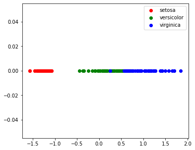
1
2
3
4
5
6
| target_ids = range(len(iris.target_names))
plt.figure(figsize=(6,5))
for i, c, label in zip(target_ids, 'rgbcmykw', iris.target_names):
plt.scatter(X_pca[y==i, 0], np.zeros(X_pca[y==i].shape), c=c, label=label)
plt.legend()
plt.show()
|
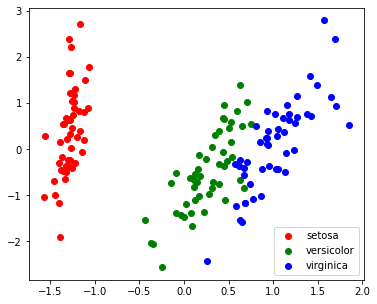
1
2
3
4
5
6
7
8
9
| pca = PCA(n_components=2, whiten=True)
pca.fit(X)
X_pca = pca.transform(X)
target_ids = range(len(iris.target_names))
plt.figure(figsize=(6,5))
for i, c, label in zip(target_ids, 'rgbcmykw', iris.target_names):
plt.scatter(X_pca[y==i, 0], X_pca[y==i, 1], c=c, label=label)
plt.legend()
plt.show()
|
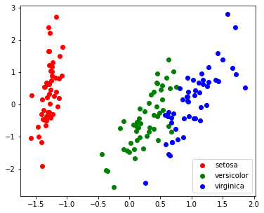
PCA Implementation
Construct a PCA function
1
2
3
4
5
6
7
8
9
10
11
12
13
14
15
16
17
| def myPCA(X:np.ndarray, n_dimensions:int):
X_centered = X - X.mean(axis=0)
Sigma = np.dot(X_centered.T, X_centered)
U, Lambda, V = np.linalg.svd(Sigma)
X_centered_PC = np.dot(U[:,:n_dimensions].T, X_centered.T).T
X_PC = X_centered_PC + X.mean(axis=0)[:n_dimensions]
return -(X_PC - X_PC.mean(axis=0))/X_PC.std(axis=0)
|
Comparison: myPCA & sklearn.decomposition.PCA
1
2
3
4
5
6
7
| X_PC2 = myPCA(X, 2)
plt.figure(figsize=(6,5))
for i, c, label in zip(target_ids, 'rgbcmykw', iris.target_names):
plt.scatter(X_PC2[y==i, 0], X_PC2[y==i, 1], c=c, label=label)
plt.legend()
plt.show()
|
1
2
3
4
5
6
7
8
9
| pca = PCA(n_components=2, whiten=True)
pca.fit(X)
X_pca = pca.transform(X)
target_ids = range(len(iris.target_names))
plt.figure(figsize=(6,5))
for i, c, label in zip(target_ids, 'rgbcmykw', iris.target_names):
plt.scatter(X_pca[y==i, 0], X_pca[y==i, 1], c=c, label=label)
plt.legend()
plt.show()
|
